Coupled-Wave Theory of Distributed Feedback Lasers
Contents
Coupled-Wave Theory of Distributed Feedback Lasers#
This page comprises simulations from the manuscript H. Kogelnik and C. V. Shank, Coupled‐Wave Theory of Distributed Feedback Lasers. Journal of Applied Physics, 43 (1972) 2327–2335. doi:10.1063/1.1661499
We compare the different simulations in the paper with our code.
Dispersion diagram for index modulation for various gain to coupling parameter ratios#
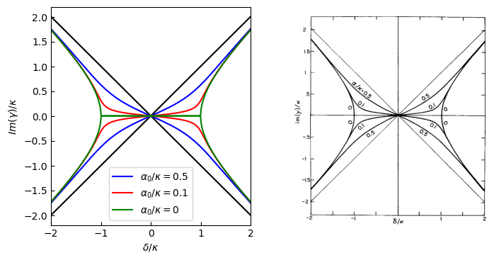
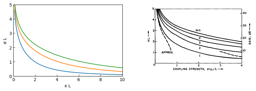
Fig. 1 (left) calculates the dispersion diagram for index modulation for various gain (\(\alpha_o\)) to coupling (\(\kappa\)) parameter ratios. In case of index modulation we have that \(\kappa= \pi n_1/\lambda_o\). We observe that the calculated result fits the result from [1], as shown in Fig. 1 (right).
Fig. 1 Left: calculated dispersion diagram for index modulation for various gain to coupling parameter ratios, right: corresponding graph from from [1]#
Dispersion diagram for gain modulation for various gain to coupling parameter ratios#
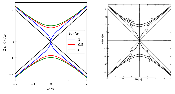
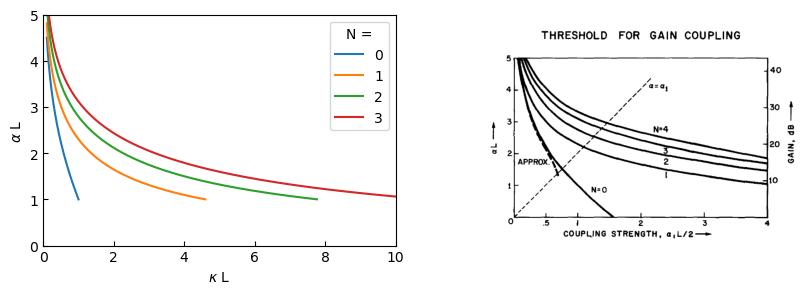
Fig. 2 (left) calculates the dispersion diagram for index modulation for various gain (\(\alpha_o\)) to coupling (\(\kappa\)) parameter ratios. In case of index modulation we have that \(\kappa= \frac{1}{2} j \alpha_1\). We observe that the calculated result fits the result from [1], as shown in Fig. 2 (right).
Fig. 2 Left: calculated dispersion diagram for gain modulation for various gain to coupling parameter ratios, right: corresponding graph from from [1]#
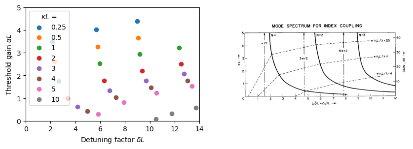
Fig. 3 Left: calculated gain required for threshold vs frequency deviation from the Bragg condition for index modulation. Only half of the spectrum is shown because of symmetry, right: corresponding graph from from [1]#
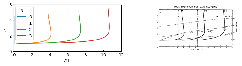
Fig. 4 Left: calculated DC gain required for threshold vs frequency deviation from the Bragg condition for gain modulation. Only half of the spectrum is shown because of symmetry, right: corresponding graph from from [1]#
Fig. 5 Left: calculated gain at threshold vs coupling strength for various modes, right: corresponding graph from from [1]#
Fig. 6 Left: calculated gain at threshold vs coupling strength for various modes. The mode number N refers to a set of modes placed symmetrically about the Bragg frequency, right: corresponding graph from from [1]#
Spatial intensity distribution of the different modes#
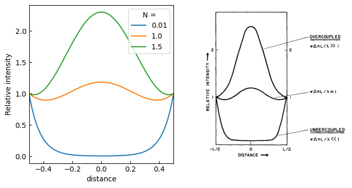
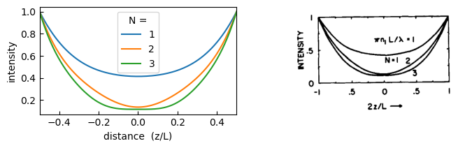
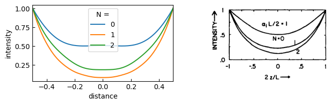
In this section we plot a few of the spatial intensity distribution of the different lowest order modes. These intensity distributions are relevant when continuous operation is targeted, as they indicate how the electrical or optical pumping needs to be distributed to maintain lasing.
Fig. 7 Left: calculated spatial intensity distribution of the lowest order modes at various coupling levels, right: corresponding graph from from [1]#
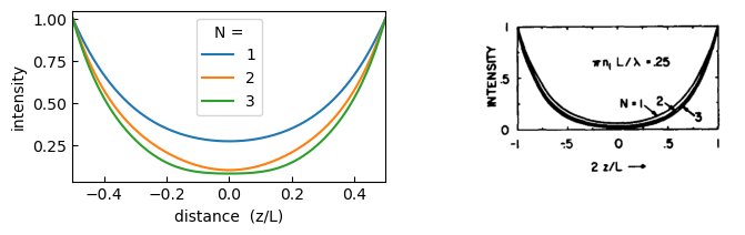
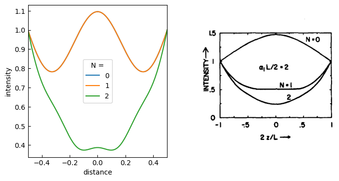
Fig. 8 Left: calculated spatial intensity distribution for the first three modes, right: corresponding graph from from [1]#
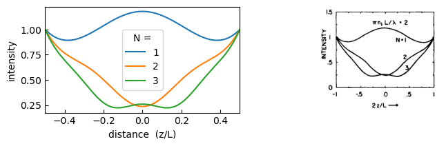
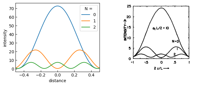
Fig. 9 Left: calculated spatial intensity distribution for the first three modes, right: corresponding graph from from [1]#
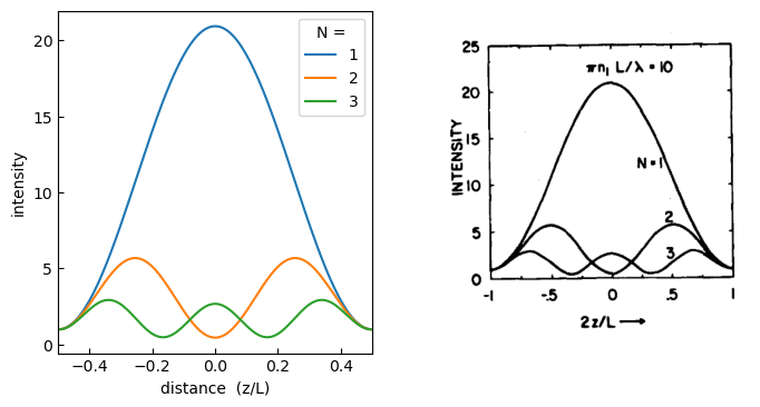
Fig. 10 Left: calculated spatial intensity distribution for the first three modes, right: corresponding graph from from [1]#
Fig. 11 Left: calculated spatial intensity distribution for the first three modes, right: corresponding graph from from [1]#
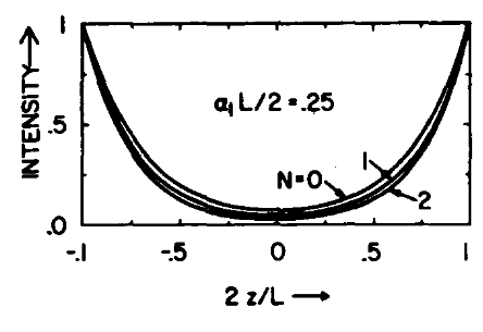
Fig. 12 Plot of the spatial intensity distribution for the first three modes at \(\alpha L / 2 =0.25\). From [1]#
Fig. 13 Left: calculated spatial intensity distribution for the first three modes, right: corresponding graph from from [1]#
Fig. 14 Left: calculated spatial intensity distribution for the first three modes, right: corresponding graph from from [1]#
Fig. 15 Left: calculated spatial intensity distribution for the first three modes, right: corresponding graph from from [1]#